VaR Based Pricing
Jump to a section1 sections in this chapter
VaR-Based Pricing
Previous chapters showed how commodity and freight traders create value through space, time and form, and how basis explains the gap between physical prices and benchmark prices. In practice, however, not every exposure can be perfectly hedged. The trader must therefore measure the residual basis risk, determine whether it remains within the company's approved risk limits, and decide what premium is required for accepting that risk. This section develops a VaR based framework for cargo positions in which traders are looking to sell freight.
Introduction to VaR
Value at RiskValue at RiskAn estimated loss threshold for a position or portfolio over a specified period and at a specified confidence level. It is not the maximum possible loss.Open in terminology, often shortened to VaR, is one of the most widely used techniques for measuring and controlling trading portfolio risk. It estimates a loss threshold over a stated time horizon and at a stated confidence level, subject to the model assumptions and data used. For example, a one day 95 per cent VaR is the loss threshold that the model expects not to be exceeded on approximately 95 per cent of trading days. It is not the maximum possible loss Frenkel, Michael and Hommel, Ulrich and Rudolf, Markus (2005).
VaR has two traditional roles for trading companies. First, it is used to set and monitor risk limits. A company can assign a VaR limit to a trader and then require the exposure to be reduced or rejected if the limit is breached. In this sense, VaR acts as a risk control tool. It tells the company whether a position remains within the approved risk limit. Research finds that traders subject to VaR limits generally take lower risk exposure than unconstrained traders and that the probability of extreme losses is also lower Cuoco, Domenico and He, Hua and Isaenko, Sergei (2008). Second, VaR creates a common denominator for comparing risk across different positions, desks and asset classes. VaR expresses their downside risk in the same monetary language. This makes it easier for top management and risk teams to compare exposures that would otherwise be difficult to assess side by side.
These two roles are especially useful in freight and commodity trading. For a route-specific freight quote, a trader may face several moving prices at the same time, including freight rates, FFA prices, bunker prices, commodity prices, foreign exchange and basis spreads. Each price can move before the trade is completed. The commercial dilemma is: if the freight quote is too high, the company may lose the customer. If the freight quote is too low, the company may accept residual basis risk without being adequately compensated for it. The framework developed here estimates the residual freight basis risk between the physical route and the selected FFA benchmark. Bunker, commodity, foreign exchange, credit and operational risks require separate measurement or risk controls. It also creates a common language between the freight, the commodity and the risk desks. The discussion therefore moves from pure “gut feeling” to a quantified discussion grounded in statistics and market fundamentals. It becomes easier to compare quotes, test against risk limits and decide whether they should be accepted, adjusted or rejected.
A Practical VaR Workflow
This chapter explains how the general VaR logic introduced above can be applied to physical quotes in freight trading. Existing research provides the main building blocks for such a framework, but generally treats them separately. The VaR literature explains how trading firms measure downside risk and use risk limits to control positions Cuoco, Domenico and He, Hua and Isaenko, Sergei (2008). The freight hedging literature studies how freight futures and FFA contracts can be used to hedge freight exposure Amir Alizadeh and Nikos Nomikos (2009). The freight basis risk literature shows that physical freight routes do not perfectly match benchmark indices, leaving residual risk remaining after hedging Roar Adland and Haiying Jia (2017).
The lack of integration between these research streams creates an important practical challenge. A trader may be able to estimate the overall freight exposure and hedge against the benchmark, but still have no systematic method for quantifying the route-specific basis risk that remains. As a result, residual risk may be under-estimated, and quote decisions may depend excessively on individual judgement rather than a transparent risk framework. This is particularly important in freight markets because even relatively small differences between a physical route and its hedging benchmark can produce losses when applied to large cargo volumes or long exposure periods. This chapter therefore proposes a practical application of VaR that connects benchmark hedging, residual freight basis risk, internal risk limits and physical pricing.
Parallel workflow for VaR based freight pricing. Branch A estimates the quote specific forward value and allowed VaR. Branch B independently estimates residual basis VaR from historical hedged basis changes. The two outputs meet at the policy gate. gives a high level map of the workflow. Steps 1 and 2 define the exposure and select the market driver. The workflow then separates into two parallel branches. Branch A estimates the forward TC rate, expected forward route basis and allowed VaR for the route and month under consideration. Branch B independently estimates the hedge ratio, historical hedged basis changes and residual basis VaR. Step 6 brings the branches together by comparing residual basis VaR with allowed VaR. If the quote passes the policy gate, Step 7 adds the residual basis risk premium and forms the final quote.
The method is organised into seven steps:
Input configuration
Market driver selection
Branch A: Forward TC, expected basis and allowed VaR estimation
Branch B: Hedge ratio estimation
Branch B: Residual basis VaR estimation
Policy gate and hedge decision
Pricing risk premium and final quote
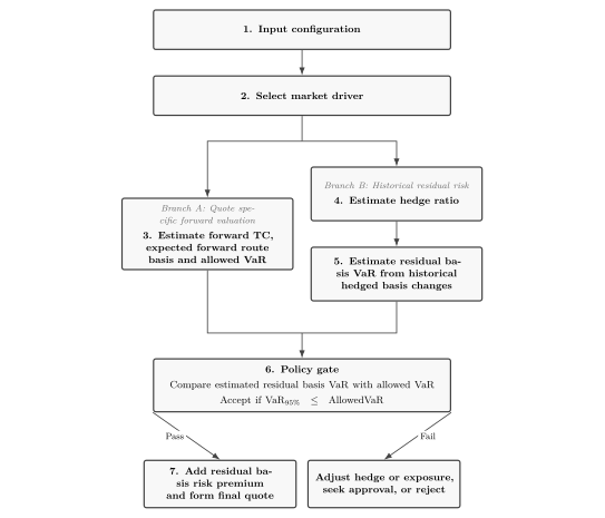
Parallel workflow for VaR based freight pricing. Branch A estimates the quote specific forward value and allowed VaR. Branch B independently estimates residual basis VaR from historical hedged basis changes. The two outputs meet at the policy gate.
Method Specification
Step 1: Input Configuration
Select the target route and TC series.
The trader first identifies the physical route to be priced and hedged. The daily TC rate for this route is expressed in USD/day.
Select the hedge month.
Next, select the hedge period, usually a calendar month denoted by . Other key parameters are all anchored to this month.
Load data inputs.
The trader then loads the required data:
Weekly historical TC assessments (USD/day) for the selected route;
Daily historical Baltic index settlements for a set of indices that could serve as candidate drivers with dates matching the weekly observations;
Current FFA forward market quotes (USD/day) for the hedge month , settling on those Baltic indices.
Step 2: Market Driver Selection
The goal of this step is to identify a market index that best tracks the target route. This index is called the market driver. Candidate drivers may include relevant Baltic route indices. To select the driver, the trader compares the historical relationship between the target TC rate and each candidate index. In practice, the Pearson correlation between the two series will be calculated for this purpose. Compared with alternative correlation measures, Pearson correlations are consistent with the linear regression framework used later, ensuring methodological consistency. However, the two series must be prepared so that their correlation reflects a stable and meaningful relationship.
Weekly to Daily TC Time Series.
Physical cash route TC assessments are in the dataset collected on a weekly basis, whereas Baltic indices and FFA prices are available on business days. To compare them, the weekly TC series must first be converted into a daily time series. The simplest approach is to carry each weekly TC quote forward until the next quote is published. For example, if the TC rate is USD/day 13,000 on 12.03.2025 and the next quote of USD/day 13,500 appears on 22.03.2025, then each calendar day in between these two dates is assigned the USD/day 13,000. This methodology impacts our results, but we consider it preferable to interpolating values between dates for the weekly observations as this would average-out the volatilityVolatilityThe degree of variation in trading prices for agricultural commodities over a period of time.Open in terminology.
Monthly Average.
The daily series is then converted into monthly averages. This reduces daily noise and makes it easier to compare the co-movement between the target TC rates and the Baltic indices. For the target route, TC quotes are carried forward until the next quote is published, its monthly average is therefore time-weighted. It means, within a given month, each quote is weighted by the number of calendar days for which it remains valid. For example, a quote valid for 10 calendar days receives a weight of 10, while a quote valid for 6 calendar days receives a weight of 6.
For Baltic indices, the monthly average is calculated as the simple average of all daily settlement prices observed during the month. In other words, each settlement is equal in weight. Non-trading days are not included because no settlement price is published on those days.
Month-over-month (MoM) Changes.
After the monthly averages of TC and Baltic indices have been calculated, both series are converted into month-over-month changes. This is because driver selection should test co-movement, not similarity in absolute price levels. A Baltic index may trade at a different USD/day level from the TC route, but it can still be a suitable driver if the two series rise and fall in a consistent way. Their month-over-month percentage changes are:
The model only compares periods where both series have valid observations. Importantly, if the effective number of observation pairs falls below a minimum threshold (for example, fewer than 12 observations for a year), the series should not be used to avoid incomplete interpretation based on fewer observations.
Rolling Correlations.
These two series of month-on-month changes are then used to calculate the Pearson correlation for selecting the market driver. However, a single full-sample correlation is not enough because the relationship between a Baltic index and a specific TC route can change over time. A hedge may work well in some years and poorly in others. For this reason, the model uses rolling correlations. Rolling correlations test whether the relationship remains stable across different market conditions rather than merely appearing strong over the full sample.
A rolling correlation calculates the correlation repeatedly over a moving time window. For example, a 12-month rolling correlation first measures their correlation over months 1 to 12, then months 2 to 13, then months 3 to 14, and so on. This produces a time series of correlation values. The trader can then see whether the relationship stayed strong, weak or broke down.
Different window lengths are used. A 12-month window is more responsive to recent market changes, but it can also be noisy. A 24-month window gives a more balanced view between recent behaviour and medium-term stability. A 36-month window is slower to react, but it gives a more robust view of the longer-term relationship. Using several windows helps avoid selecting a driver that only looks good in one test. A good driver should perform reasonably well across short, medium and longer windows. The correlation calculation is therefore repeated over 12-, 24- and 36-month rolling windows.
Driver Selection Rule.
The driver is selected by comparing the rolling correlation results across all candidate indices. A good driver should meet two conditions: it should exhibit both a high correlation with the TC route and this correlation should be stable across the 12-, 24- and 36-month windows. In practice, the trader compares the average rolling correlation, the variability of that correlation, and the recent correlation trends. The preferred driver is the index that moves most closely and most consistently with the physical route.
The framework uses historical prompt month values because it assumes that the freight position remains open until physical execution. For quotes made well before execution, the calibration should instead use historical FFA contracts with a remaining tenor comparable to the position being priced.
Step 3: Forward TC, Basis and Allowed VaR Estimation
Historical Levels Regression.
Once the driver index has been selected, the next step is to estimate how the target TC rate has historically priced relative to that driver. This step uses the same TC and driver series in daily level form as introduced in Step 2. Let denote the historical TC rate (USD/day) for the target route on business day and denote the daily level of the selected driver index on the same day. The model estimates this relationship with a simple linear regression as:
The coefficient measures how strongly the TC rate tends to move with the driver in levels. For example, if =1.20, a USD 1,000/day increase in the driver has historically been associated with an average USD 1,200/day increase in the target TC route. Historical relationship between route TC and selected Baltic driver. illustrates this estimate. Each dot is an observed pair of route TC and driver level. The fitted line shows the average historical relationship between them. The slope of the line is .
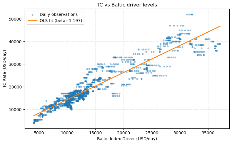
Historical relationship between route TC and selected Baltic driver.
Forward TC Estimation.
The regression equation above describes the historical relationship between the target TC route and the selected driver. The next step is to apply this relationship to the forward market. The selected FFA contract provides a forward market price for the driver. The trader can therefore use the FFA quote as the forward input in the model. Let denote the current FFA quote for month , implying the forward level for that driver. By inserting into the regression equation, the model estimates the forward TC rate for the target route:
Here, is the model-estimated forward TC rate, not a guaranteed market price. This projection assumes that the historical relationship between the target route and the FFA index remains informative for the hedge month. The estimation should therefore be reviewed when structural or market conditions differ materially from the historical period.
Expected Forward Route Basis.
The expected forward route basis is defined as the difference between the model-estimated forward TC rate for the target route and the current FFA quote for the selected driver:
A positive expected forward basis means that the target route is expected to price above the FFA benchmark. A negative basis means the target route is expected to price below the FFA benchmark. The basis is expressed in USD/day.
Allowed VaR.
The expected forward route basis is then converted into a quote specific policy limit. Let denote the company's risk budgetRisk budgetThe amount of risk allocated to a strategy or desk, often expressed as a VaR limit or loss limit.Open in terminology parameter. The allowed VaR is:
The expected forward route basis is used as the scaling reference because it represents the expected difference, in USD/day, between the physical route and the FFA benchmark for the route, month and quote under consideration. The parameter specifies the proportion of this expected difference that the company is willing to accept as residual basis risk.
For example, if , the allowed VaR equals 10 per cent of the absolute expected forward route basis. This scaling rule is an internal policy choice rather than a statistical relationship between expected basis and residual volatility.
Where the company also applies an absolute daily cap , the policy limit becomes:
Step 4: Hedge Ratio Estimation
The forward TC rate has now been estimated for the physical route. The next question is how this exposure should be hedged. The challenge is that the FFA contract does not settle against the trader's exact physical route. It settles against the selected Baltic index. In other words, the trader is using a related paper market to hedge a physical freight exposure. Two markets are related but not identical.
This is why the hedge ratio is needed. It shows how strongly the physical route has historically moved when the selected Baltic index moves. For example, suppose that the Baltic index moves by 1,000 USD/day, while the physical route usually moves by USD 1,500/day. A one-for-one hedge would be too small because the FFA hedge would offset only 1,000 USD/day of movement, while the physical route moved by 1,500 USD/day. The trader would still be left with 500 USD/day of unhedged movement. In that case, the hedge ratio would be 1.5. If the physical route usually moves less than the index, the hedge ratio would be below 1, and the trader would use less FFA exposure. The purpose of the hedge ratio is therefore to make the FFA hedge more proportional to the physical exposure. A good hedge ratio reduces the day-to-day volatility of the hedged TC position's profit and loss (P&L).
Daily Changes.
To estimate the hedge ratio, the model must compare movements in the physical route with movements in the selected driver. This step also uses a regression between the TC rate and the driver index, but the purpose is different from Step 3. Step 3 used price levels to estimate the forward TC rate level. Here, daily changes in the TC and the driver index are used to estimate the hedge size. This is because hedging is about offsetting movements in profit and loss (P&L), not estimating the price level.
Let and denote the daily levels of the TC rate and the driver index, aligned on a common set of business days. The daily change is measured as the difference between today's value and the previous period's value:
Hedge Ratio.
The hedge ratio, denoted by is estimated as the slope in the regression of daily TC changes on daily driver changes:
Note that forward-filled TC observations are excluded from the regression because they do not contain new market information and would otherwise generate artificial zero changes in .
This slope measures the historical conditional co-movement between changes in the physical TC rate and the changes in the driver. When applied to hedge sizing, tells the trader how much FFA exposure is needed for a given amount of physical TC exposure. If the trader has 100 vessel-days of physical TC exposure and =1.5, the model suggests hedging with 150 vessel-days of FFA exposure. In practical application, a common choice is to estimate the hedge ratio over a rolling window of recent history (for example, the last 252 to 520 business days) to reflect current market dynamics.
Step 5: Residual Basis VaR
Hedged Basis Change.
After hedging based on the estimated hedge ratio, the next step is to measure the risk that the hedge did not capture. The model therefore calculates the hedged basis change:
where and are the daily changes defined in Section [HedgeRatio]. The represents the movement offset by the FFA hedge. Their difference is the hedged basis change. The model uses daily changes rather than price levels because a high or low basis level does not create a daily gain or loss. It comes from how the basis changes from day to day.
For a freight buyer, a positive value of represents a loss because the physical TC cost has increased more than the hedge has offset. A negative value indicates a profit because the physical TC cost has fallen or the hedge has more than offset the increase. The daily loss is therefore defined as:
Accordingly, represents a loss (in USD/day) on day , and represents a gain.
One-day Residual Basis VaR.
VaR has a statistical definition. For a loss variable, the VaR at confidence level is the empirical quantile of loss distribution at level Giot, Pierre and Laurent, S\'ebastien (2003). In other words, VaR identifies the loss threshold that is not exceeded in percent of the historical observations.
The previous step constructs the historical daily loss variable , where positive values represent losses and negative values represent gains. This historical distribution of (for example the most recent 500 observations) is used to calculate the VaR directly. This approach is called historical simulation VaR because the model uses the historical distribution of , rather than assuming a specific statistical distribution. More specifically, the historical outcomes are ranked from smaller to larger values, and the model identifies the loss threshold linked to the chosen confidence level, for example 95 percent.
It is a one-day residual basis VaR because is constructed from daily hedged basis changes. Because losses are recorded as positive numbers, the one-day 95 percent residual basis VaR is the 95th percentile of the historical loss distribution:
This means the loss threshold was not exceeded in approximately 95% of historical observations. Equivalently, approximately 5% of the observations produced a larger loss. If the one-day 95% residual basis VaR is USD 1,000/day, then approximately 95% of the historical daily losses were no worse than USD 1,000/day, while approximately 5% were worse. It is worth noting that provides a historical estimate of the residual risk associated with the selected hedge relationship over the chosen estimation period, rather than for the individual quote itself.
The VaR reported here is expressed in USD/day, because it measures the residual basis risk per unit of freight exposure. For a specific trade, this rate based VaR can be converted into a monetary VaR by multiplying it by the number of vessel days represented by the physical and FFA exposure.
Diagnostic distribution of the historical basis.
The distribution of historical basis may be asymmetric and may exhibit heavy tails. As a sense check, the trader may also examine the historical pattern of daily basis in levels.
Figure Empirical distribution of historical basis levels between the physical route and the selected Baltic driver. shows how often the historical basis outcomes fell within a certain range. If most observations are close to the centre, the basis is relatively stable. If the distribution is wide, the basis has moved more sharply. The density curve is the smooth line drawn over the histogram. It shows the same information in a smoother way. The combination of histogram and density gives both a discrete and a continuous view of the typical size and dispersion of the basis, providing economic intuition that complements the one-day .
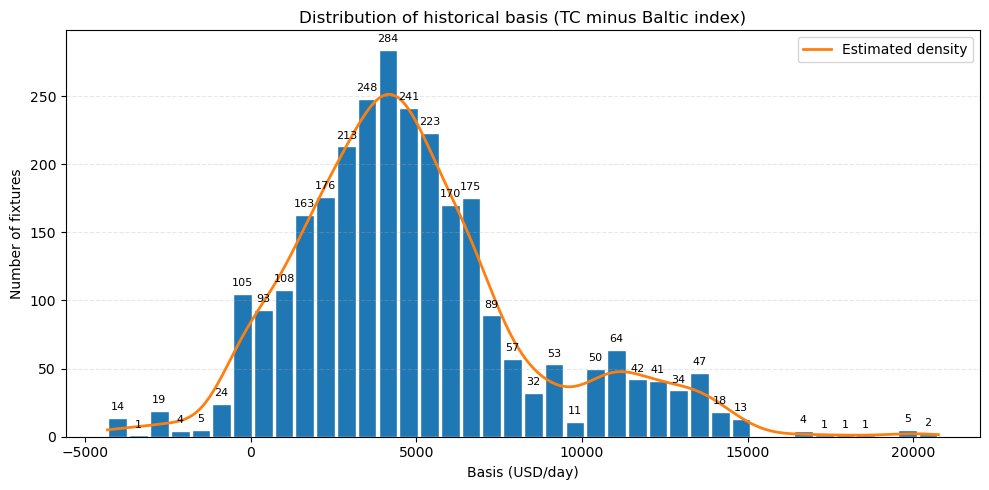
Empirical distribution of historical basis levels between the physical route and the selected Baltic driver.
Step 6: Policy Gate and Hedge Decision
The policy gate brings the two branches together. Branch A provides the quote specific allowed VaR calculated in Step 3. Branch B provides the historical residual basis VaR estimated in Step 5. Step 6 compares these two values to determine whether the proposed hedge and exposure remain within the company's policy limit.
Hedge Decision Rule.
Let denote the one-day 95 percent residual basis VaR estimated in Section [hedgedBasis]. This residual basis VaR provides a historically-based estimate of the residual risk associated with the selected hedge relationship over the chosen estimation period. It is assumed that the historical distribution of the hedged basis changes remains representative of the residual basis risk likely to be faced by the quote under current market conditions. Under this assumption, serves as a proxy for the prospective residual risk of the quote and can therefore be compared with the quote-specific allowed VaR.
Subject to this assumption, the estimated residual basis risk at 95 percent confidence level is tested against the company's quote-specific policy gate:
if , the expected residual risk of the quote is within the company's risk limit for that quote. The hedge therefore passes the policy gate;
if , the estimated residual risk of the quote exceeds the company's risk limit for that quote. The hedge therefore fails the policy gate and must be adjusted or rejected.
A quote is accepted only if hedged VaR sits below the policy line. provides a simple visual introduction to this policy gate. The x-axis shows the expected forward route basis, expressed in USD/day. The y-axis shows the one-day residual basis VaR, also expressed in USD/day. Each quote becomes one point. The sloping policy line represents the allowed VaR. In this example, the risk budget . The green point below the line passes the policy gate because the VaR is within the approved limit. The red point above the line fails the policy gate because the VaR is too high.
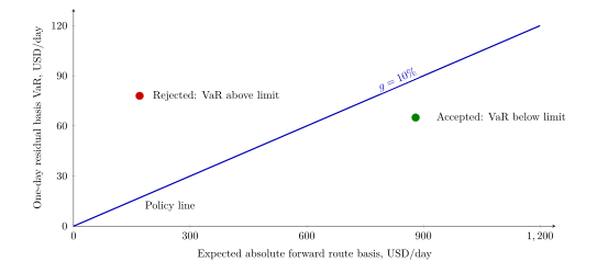
A quote is accepted only if hedged VaR sits below the policy line.
In cases of failing the policy gate, the desk may reduce the residual basis risk through various options including, but not limited to:
selecting a more suitable hedge instrument if the current FFA index does not track the physical route closely enough;
changing the FFA tenor if the hedge month does not match the physical exposure period;
reducing the physical exposure by lowering the cargo size, vessel-days or other commitment;
splitting the exposure across more than one hedge if no single index sufficiently captures the route risk;
seeking manual approval by management or risk management team if the trade remains commercially attractive despite the policy breach.
Route Example
The following example uses the seven-step framework for a single Handysize route and forward month using internally consistent placeholder numbers as a numerical illustration of the model's use. In implementation, all quantities are read directly from the production data and notebook. Assume we are in October 2025.
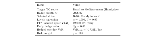
Inputs for the Handysize route hedging example.
Step 1–3 (Driver and Forward TC Estimate): Using the levels regression, the forward TC for the target physical route in month , based on the FFA quote for the selected Baltic Handy index is:
The expected forward route basis is then calculated as the difference between the model-estimated forward TC rate and the FFA benchmark:
This means that the target physical route is expected to price USD 900/day above the selected driver.
Step 4–5 (Hedged Basis and VaR): Based on historical daily changes in TC and the selected driver, the daily hedge ratio is estimated as . The model then constructs the hedged basis change:
The daily loss variable is therefore:
Using the historical distribution of loss series, the model estimates a hedged one-day 95 percent VaR of:
.
Step 6 (Policy Gate and Hedge Decision): With a risk budget parameter of , the allowed daily VaR is
Since , the hedge sized at is accepted under the policy gate.
Step 7 (Pricing Risk Premium):
Because the quote passes the policy gate, the company can move from risk control to pricing. The residual basis risk premium is:
Suppose that . The residual basis risk premium is therefore:
The final TC quote is:
Governance and Model Use
Model governance should be built around repeatable actions, documented assumptions and transparent exception handling. The example below is a stylised governance framework adapted from commodity trading practice. It is illustrative and should not be interpreted as standard practice across all shipping companies.
A freight desk could rerun the calibration and VaR computation daily, refreshing the regression window, forward curve snapshot and empirical loss distribution. The model policy should define which changes in coefficients or VaR outputs are material and specify when commentary or approval is required. For example, a change of more than 15 per cent in the hedge ratio could trigger documented analyst review. Traders may exercise commercial judgement on individual quotes only within approved desk limits and exception procedures. They may not exceed the total VaR limit for the trading book without formal approval.
An independent risk department performs deep dives at a defined interval that include back testing of the hedged VaR, stress testing the regression under alternative driver selections, and validation that liquidity thresholds were respected. Scenario libraries covering macro shocks such as fuel price spikes or canal disruptions are periodically refreshed and replayed across the archived hedged basis to confirm resilience. When data gaps or thin FFA liquidity arise, the desk escalates to a manual approval process rather than forcing the model to produce a number. Training notes, governance meeting minutes, and remediation plans are circulated so that process knowledge survives analyst rotation. All artefacts—input data, code versions, regression diagnostics, VaR charts, and hedge instructions—are stored for at least one year to meet internal and regulatory retention policies.
Limitations and Cautions
The method inherits the usual limitations of historical-simulation VaR: structural breaks, regulatory shocks, and shifts in fleet deployment can render the past an unreliable guide to the future. Stochastic freight models emphasise the potential for regime changes and volatility clustering, so users should monitor whether the empirical loss distribution shows signs of instability or heavy tails beyond the chosen quantile Fred Espen Benth and Steen Koekebakker and Che Mohd Imran Che Taib (2015). Incorporating scenario analysis, regime classification dashboards, and expected shortfall metrics is recommended when policy frameworks evolve or when management raises concern about tail alignment with corporate stress tests.
Linear hedge scaling delivers intuitive closed-form expressions but can misstate risk when the regression fit deteriorates or the hedge tenor diverges materially from the voyage exposure. In such cases, practitioners should recompute hedged VaR directly, explore multi-instrument hedges, and layer execution cost add-ons before signing off on a quote Marcel Prokopczuk (2011). Desk users must also be mindful that execution slippage, settlement mismatches, and counterparty credit deterioration are not explicitly modelled; these factors require overlays, possibly in the form of add-on reserves or separate credit valuation adjustments. Finally, the framework assumes that operational logistics (port congestion, bunker delays, laycan adjustments) can be captured through deterministic exposure adjustments, i.e. converting an operational risk into a fixed assumption rather than modelling it as an uncertain distribution. When these assumptions fails the VaR gate should be complemented with scenario-based contingent cash flow modelling.
Future Work
Further development can enhance robustness and strategic insight across the modelling chain. Possible extensions include:
Driver selection: evaluate Bayesian model averaging or sparse machine learning screens to capture multi-factor driver structures while controlling for overfitting.
Regression dynamics: investigate state-space or regime-switching regressions that allow and to adapt to structural shifts in freight markets.
Basis modelling: augment the linear scaling assumption with nonparametric bootstrapping or copula-based dependence structures between TC and FFA series.
Risk metrics: complement VaR with expected shortfall, drawdown statistics, or filtered historical simulation to better capture tail persistence.
Hedge optimisation: replace the static hedge ratio with a stochastic programming formulation that includes liquidity, execution costs, and cross-instrument hedges.
Quote strategy: extend the pricing module to evaluate option overlays (e.g., caps/floors) or customer-specific discount curves that optimise expected margin under VaR constraints.
Portfolio optimisation: Using expected shortfall models could allow the trader to look at multiple positions from a portfolio point of view, i.e. a hypothesis could be that having both Atlantic and Asian cargo exposures partly offset each other's residual basis risk.
Definitions and notation
This section summarises the notation used in the hedging framework. Table Core time-series variables and derived quantities lists the core time-series variables and derived quantities, while Table Model parameters and policy inputs collects the main model parameters and policy inputs.
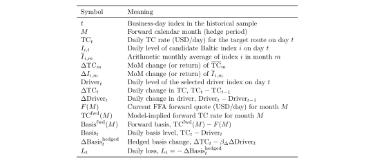
Core time-series variables and derived quantities
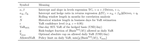
Model parameters and policy inputs
Carry the model forward.
Key Takeaways
Pricing should reflect both the trader's market view, market competitiveness and the firm's approved risk budget.
VaR-based pricing is most useful when it is transparent, auditable and easy to communicate across desks.
Hedging reduces but does not eliminate basis risk; accepted residual risk should inform pricing.
A model should be treated as a disciplined decision aid, not as a substitute for judgement.
Epilogue
The Epilogue reconnects the pricing framework to the book's central argument: freight belongs inside the trade from the first commercial decision.
Continue to Epilogue