Space, Time and Form
Jump to a section10 sections in this chapter
Balance Sheets introduced balance sheets as a way to understand the supply and demand balance in the market. A balance sheet can show the market imbalance, but it does not automatically create profit. The trader's next task is more practical: transform this market imbalance into a margin.
A commodity trader rarely earns a margin simply by buying and selling the same product in the same place at the same time. Value is created by transformation: moving a commodity from surplus to deficit regions, holding it from periods of abundance to periods of scarcity, or changing its quality, specification or contractual form so that it better fits buyer demand. This is the practical heart of physical commodity trading and the same logic applies in freight trading. This leads to the core of this chapter: the transformation marginTransformation marginThe expected value after transformation, less the value before transformation, execution costs and the required risk allowance.Open in terminology.
The Transformation Margin Framework
Transformation margin provides a practical framework for deciding whether a trader should act on a market imbalance. Expected transformation margin = value after transformation - value before transformation - execution costs - risk allowance
The formula captures the commercial logic behind many physical trading decisions. It asks whether the trader can improve a position enough to justify the cost, time and risk required to do so. Value after transformation is the expected value of the physical position after the trader has changed it. This could be the value of grain delivered to an import port, the value of a cargo sold later in the season, or the earnings of a vessel after repositioning into a stronger freight market. Value before transformation is the current value of the position. This may be the origin cash price of the cargo, the value of the cargo in its current quality or the current employment value of a vessel. Execution costs are the costs required to complete the transformation. In commodity trading, these may include freight, storage, finance, insurance, blending, inspection and port charges. In freight trading, they may include bunkers, ballast costs, waiting time, commissions and the opportunity cost of using a vessel on one route rather than another. Risk allowance is the margin a trader requires in case execution conditions change or other problems arise before the trade is complete. A cargo may fail specification. A buyer may delay payment. The risk allowance is the extra margin a trader requires to justify these uncertainties.
The formula bridges market diagnosis and physical trading, and therefore can be read as a decision rule. It prevents the trader from looking only at the headline price difference. Before committing capital, the trader must ask: Is the expected value gained from transformation greater than the full cost and risk of making the transformation?
The transformation formula can be applied through space, time and form. They are the three practical levers through which traders turn a market imbalance into a more valuable commercial position, thus creating value. Space refers to location: a commodity or vessel may be worth more in one place than another. Time refers to timing: a cargo, freight exposure or vessel position may be worth more in a future period than today. Form refers to the physical, contractual or commercial shape of the position: the same underlying commodity or freight exposure may have a different value once its quality, specification, delivery terms or contract structure changes. Despite the logic remaining the same, each lever has its own formula variation of transformation margin:
Space transformation margin = destination value - origin value - transport and logistics costs - risk allowance
Time transformation margin = future value - current value - carrying costs - risk allowance
Form transformation margin = adjusted value - original value - processing and operational costs - risk allowance
Transformation in Commodity Trading
Space transformation refers to reallocating commodities from regions with surplus to areas with shortage. Commodity production is geographically concentrated and often distant from urban centres where demand is dispersed. Bridging this imbalance requires efficient logistics to move wheat from farms to mills and markets. This spatial adjustment is crucial for the functioning of the supply chain and the global food economy. Traders and logistics providers coordinate this movement, optimising routes and managing transportation costs. By coordinating freight, traders also transform regional imbalances into arbitrage opportunities. Moving commodities is what freight is about, hence this section will be short as the rest of the book should cover all the necessary challenges and opportunities in freight trading. Commodity trading is essentially a transformation business. Traders create value by using one or more types of transformations. When these transformations are used to capture a price difference between two physical conditions of the commodity, the activity can be understood as physical arbitragePhysical arbitrageAn executable trade that captures a price difference between physical states after transport, storage, finance, processing, operational costs and risk are included.Open in terminology Craig Pirrong (2018).
Space, time, and form in physical commodity arbitrage frames physical arbitrage as an ongoing three-dimensional optimisation problem across space, time and form. The trader's core task is to choose the combination of location, timing and form that maximises net margin.
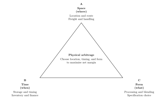
Space, time, and form in physical commodity arbitrage
In Space
Space transformation in commodity trading is about whether a geographical price spread can be physically captured. A commodity is generally and logically cheaper in a surplus origin and more expensive in a deficit consumption region, but the spread is only tradable if the cargo can be moved through the required supply chain Luc Nijs (2014). For grain, this may mean moving wheat from inland farms to mills or export markets. For energy commodities, it may mean moving biomass, coal or crude oil from production areas or refineries to regions where demand is. The commodity trader's task is to examine whether the price spread is large enough to cover transport and logistics costs, as well as execution risk. If so, they will coordinate this movement, optimising routes and managing transportation costs.
In Time
Time transformation in commodity trading is about deciding when a physical commodity should be released into the market. Many commodities are produced or harvested in uneven flows, while consumption is more continuous. For example, wheat harvests occur seasonally, often once a year, but its consumption is continuous throughout the year.
Storage gives traders flexibility over when inventory enters the market. Instead of all production being sold immediately when it is harvested or produced, part of the flow can be held back and released later according to market conditions. In this sense, storage works like a tap: traders can slow or increase the release of inventory in response to prices, demand, logistics constraints and expectations about future supply. This is how storage links today's spot market with the market of the future, by continually comparing the value of selling now with the value of carrying inventory forward.
This is especially important for storable commodities such as wheat, corn, soybeans, peanuts, crude oil and natural gas. The trader's decision is not simply whether storage is available, but whether storage is profitable. Holding inventory ties up capital and creates storage costs, financing costs, handling costs into and out of storage, insurance costs and quality deterioration risk Helyette Geman (2015). For grain, this may also include shrinkage or moisture problems. For oil and refined products, tank availability and financing cost can become key binding constraints.
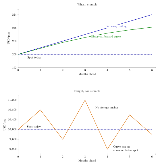
Storability links spot and forward prices for wheat through carry, while freight has no storage anchor. In the top panel, the dashed line is today’s spot price, the blue line is the full carry ceiling and the green line is the observed forward curve. The top panel is in USD/pmt and the bottom panel is in USD/day.
In Storability links spot and forward prices for wheat through carry, while freight has no storage anchor. In the top panel, the dashed line is today’s spot price, the blue line is the full carry ceiling and the green line is the observed forward curve. The top panel is in USD/pmt and the bottom panel is in USD/day. one can see why storability matters for time transformation. The top panel shows wheat, a storable commodity. The dashed horizontal line is today's spot price. The blue upward sloping line is the full carry ceiling over time, which represents the spot price plus storage, finance, insurance and other carrying costs. The green line is the observed forward price.
If the observed forward curve is above today's spot price, the market is in contango. Storing wheat may be profitable if the deferred premium is high enough to cover the trader's actual carrying costs. If the observed curve is below today's spot price, the market is in backwardation and storage is less attractive. Inventory holders are encouraged to sell promptly, while buyers may lock in lower deferred prices through forward or futures contracts. Neither curve should be interpreted as a prediction that the future spot price will necessarily equal the current forward price.
The bottom panel of Storability links spot and forward prices for wheat through carry, while freight has no storage anchor. In the top panel, the dashed line is today’s spot price, the blue line is the full carry ceiling and the green line is the observed forward curve. The top panel is in USD/pmt and the bottom panel is in USD/day. shows freight as the contrast case. Unlike grain and oil products, which can generally be stored, freight and electricity cannot be stored economically for later sale. For that reason, the orange forward curve fluctuates above and below spot prices. The figure shows why wheat and freight require different forward pricing logic: wheat is anchored by carrying costs, while freight cannot be stored. Withholding freight capacity requires a vessel to remain unemployed for a period, which is normally uneconomic. In periods of very low rates, however, owners may lay up vessels when they judge this to be the best available economic option. Taking vessels out of service reduces active supply and may contribute to a later recovery in rates.
In Form
Form transformation refers to the processing of raw commodities into products with enhanced utility and value. It represents the vertical dimension of commodity trading, where value is created not by movement or storage, but by conversion. It changes what the cargo effectively is and increases its market value, by altering the physical or chemical state of commodities to meet market demands, comply with industry standards and cater to consumer preferences.
Take wheat as an example. Raw wheat grains have limited direct consumption but serve as the foundational input for many other products. Milling wheat transforms it into flour, the primary ingredient for bread, pasta, pastries and other staples. This transformation not only changes the grain's form but also increases its market value by making it suitable for a variety of food products. Wheat can also be processed into starch, gluten and even biofuels. Each of these derivatives requires specific processing methods and caters to different market segments. Each derivative product competes for the same supply, so traders and processors in general calculate processing margins across alternative uses and whatever returns the highest PnL, and is therefore able to pay the highest price, takes the supply.
Trading firms play a pivotal role in facilitating form transformations. They coordinate sourcing, processing capacity and logistics, ensuring that raw materials are allocated to the highest-value sector and usage. For trading decisions, the trader compares the price of the processed forms with the cost of input raw commodity, processing expenses and risk adjustment.
Given a fixed amount of input commodities, traders and processors may use linear optimisation models to maximise profits. For example, a milling company might use linear programming to determine the optimal mix of wheat varieties to produce different types of bread, considering constraints like processing capacity, input costs and market prices. Competitive dynamics further influence these decisions, as firms must anticipate capacity expansions, technological upgrades and pricing strategies of rivals.
Freight pricing is another crucial element influenced by form transformation. Processed goods often have different transportation requirements, e.g. container transportation, which compared to the transport of raw commodities is in general more expensive than bulk transport. For example, flour may require more stringent handling and storage conditions than wheat grains to prevent spoilage and contamination. These factors affect freight costs, which must be incorporated into overall form-margin calculation.
Applied example: Fertilizer blending and freight in West Africa
Form transformation in fertiliser trade means blending standard nutrient products into a crop- and soil-specific grade. Nitrogen can be supplied through urea, phosphorus through diammonium phosphate (DAP) or monoammonium phosphate (MAP), and potash through muriate of potash (MOP). The commercial value comes from converting separate inputs into a fertiliser mix that better matches local demand.
Consider the phosphate producer OCP as a case study. It mines phosphate rock in Morocco, converts it into products such as phosphoric acid, and produces DAP, MAP and NPK fertilisers. In West Africa, OCP's model treats DAP not only as a finished product but also as a phosphorus base that can be combined with other nutrients closer to the buyer and sold at a premium Kristin Fabbe and Forest Reinhardt and Natalie Kindred and Alpana Thapar (2018).
Different crops require different recipes. Corn may require more nitrogen to support growth. Cocoa may require more potash, while cotton may require a different balance of nitrogen, phosphorus, potash and micronutrients. OCP has developed formulations for maize and cocoa in Nigeria, and for cotton in several West African markets. The trader is therefore converting their form so that the final product matches local soil and crop demand.
A simple example is 100 tonnes of fertiliser. This means the finished blend must contain 15 percent of nitrogen, 15 percent of phosphate and 15 percent of potash. Therefore, the finished blend needs 15 tonnes of each.
DAP contains about 46 percent phosphate. To supply 15 tonnes of phosphate, the blender therefore needs about 33 tonnes of DAP. DAP also contains nitrogen. The 33 tonnes of DAP provide about 6 tonnes of nitrogen. The blend still needs another 9 tonnes of nitrogen. Urea contains about 46 percent nitrogen. To supply the remaining 9 tonnes of nitrogen, the blender needs about 20 tonnes of urea. MOP contains about 60 per cent potash. To supply 15 tonnes of potash, the blender needs 25 tonnes of MOP.
The remaining 22 tonnes consist of carrier material, such as limestone or gypsum. This brings the blend to 100 tonnes and helps achieve the required nutrient concentration and handling quality. This brings the recipe as follows:
The precise commercial recipe may differ slightly because nutrient assays, moisture, secondary nutrients, micronutrients and blending tolerances must also be considered.
The example also shows why form transformation cannot be separated from space and time. DAP may come from Morocco, while urea can be sourced from the Middle East, China, Russia or a local producer. The cheapest FOB urea is not necessarily the cheapest delivered input. A Chinese offer may be attractive on FOB, but the longer sailing time can increase freight exposure and create a risk of missing the planting window. A closer origin may cost more FOB but arrive earlier and reduce execution risk.
Freight therefore shapes the blending plan. A large programme may justify a full Handysize or Supramax of one grade, lowering freight cost per tonne. Smaller and more varied demand may justify mixed parcels. Once products are assembled at one load region or hub, a five hold geared vessel might carry DAP in holds one and two, MOP in hold three, and urea in holds four and five. At destination, each product is discharged separately, stored, tested, blended and bagged. Full ships provide scale. Mixed parcels cost more, but preserve flexibility to make the right blend for the right crop at the right time.
Transformation in Freight Trading
Freight trading is different from commodity trading in the details, but overall it operates within the same space-time-form dimension. Traders seek to maximise profits by strategically manoeuvring vessels and transforming transport capacity. Understanding these dimensions is crucial for navigating the complexities of maritime markets and capitalising on emerging opportunities, even if freight rates are shown to be globally mean reverting over the long-term Roar Adland and Kevin Cullinane (2006).
Simplified value chain for agricultural freight trading places the space-time-form framework inside a commodity freight value chain, from FOB origin to CFR destination. The figure shows that freight is the central space transformation. Transformations in time and form may occur before loading, during the export process, or at destination.

Simplified value chain for agricultural freight trading
In Space
Space is the primary arena for freight traders Roar Adland and Fredrik Bjerknes and Christian Herje (2017). Value is created by positioning vessels from low-earning regions to high-earning ones Risto Laulajainen (2007). Traders constantly monitor global trade flows, economic indicators and geopolitical events to predict where demand for shipping capacity will increase (and where it will not!).
For instance, a surge in soybean exports from Brazil to China, such as during periods of trade tension between USA and China, increases demand for bulk carriers in the South Atlantic. Freight traders anticipating this shift may ballast bulk carriers towards South American loading regions before the export peak, in order to capitalise on the expected premiums during peak export seasons.
Advanced technologies, such as AIS data, enable traders to track vessel movements in real-time. This information allows them to make informed decisions about where to allocate their fleet. Combined with regional supply-demand balance sheets, this information allows traders to estimate whether a spatial premium justifies the repositioning investment.
However, space can also be a restriction on trade in the sense that a blockage can make it much more expensive to deliver goods. The Strait of Hormuz is a good example of such a choke point. A party blocking this strait can make it difficult, if not downright impossible in the quantities needed, to supply the world with e.g. fertiliser and oil in the volumes expected prior to a blockade. Traders solve these problems either by finding alternative sources of supply or finding out at what price point demand destruction occurs.
Theoretical spatial transformation from FOB purchase to CFR sale turns this spatial decision into a simple margin test. The trader starts with the FOB price at origin and adds ocean freight, insurance, finance and documentation to calculate the landed cost at destination. This landed cost is then compared with the expected CFR sale price from the destination buyer. The trade is normally attractive only when the expected CFR sale price leaves enough margin to compensate for execution risk and provide the required profit. However, the initial CFR sale may have a negative margin if the trader expects the value of the resulting optionalityOptionalityOptionality in commodity supply chains provides flexibility to adapt sourcing, logistics and delivery routes based on market conditions, costs, or demand shifts. This adaptability helps manage risks and capture pricing advantages.Open in terminology to exceed that loss.
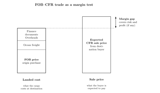
Theoretical spatial transformation from FOB purchase to CFR sale
In Time
Timing is another critical dimension in freight trading Z. S. Zannetos (1966). Unlike commodity traders who store inventory to arbitrage time, freight traders cannot store transport capacity. Instead of storage, freight time arbitrage is achieved through scheduling and contract structuring. Traders aim to synchronise vessel availability with anticipated demand peaks in order to secure higher freight rates. This requires precise forecasting to ensure that vessels reach their destinations at the most advantageous times. For example, a freight trader anticipating a spike in fertiliser exports from the Arabian Gulf can schedule vessels to arrive shortly before the expected increase in cargo volume. Arriving too early may result in waiting time and opportunity cost; arriving too late means missing the premium.
However, timing strategies are inherently risky. Weather disruptions, port congestion and unexpected changes in market conditions can quickly erode expected gains Roar Adland (2003). As freight capacity is perishable, timing deviations translate directly into lost earnings.
The timing dimension is influenced not only by macroeconomic conditions but also by contract characteristics at the micro level. Amir Alizadeh and Wayne K. Talley (2011) demonstrate, using a large sample of individual dry bulk charter contracts from January 2003 to July 2009, that laycan duration affects dry bulk freight rates. A longer laycan may provide flexibility but typically has different pricing from a tight loading window, reflecting the value of timing.
Effective time transformation therefore combine elements of forecasting, assessment of contractual flexibility and risk management, all done under uncertainty. Unlike commodity storage decisions, which smooth supply over time, freight timing decisions attempt to match mobile capacity with temporary demand spikes.
In Form
While space and time dominate short term vessel deployment, form determines which employment choices are available to the vessel. In freight trading, form has both a physical and a contractual dimension.
Physical form refers to the characteristics of the vessel. Size, gear, hatch strength, tank top strength, hold condition, draft, ice class, age, fuel efficiency and emissions status determine which cargoes the vessel can carry and which ports it can enter. A geared vessel can serve ports without shore cranes. A vessel with suitable hatch and deck strength may carry project cargo on one leg and grain on a later leg. These characteristics widen or narrow the vessel's available employment set.
Contractual form determines how the vessel can be employed and how costs, control and flexibility are allocated between the parties. A voyage charter, trip time charter or period charter may involve the same vessel, but each contract creates a different economic exposure. Under a voyage charter, the owner normally bears bunker, port and duration risk. Under a time charter, the charterer normally pays the voyage costs and directs the vessel within the agreed trading limits. Redelivery ranges, cargo exclusions, cancellation dates and notice periods also affect where and when the vessel becomes available for its next employment.
Most physical vessel characteristics are fixed over the spot trading horizon. An owner cannot change the vessel's size, gear or fuel consumption simply because another cargo pays more. Over a longer horizon, the owner may alter form through retrofits, technical upgrades or changes in fleet composition. The investment is justified only when the expected value of the additional employment choices exceeds the cost of creating them.
Form therefore matters because it determines which employment chains are feasible. A vessel may be positioned in the correct region at the correct time, but still be unable to perform the available cargo because its technical or contractual form is unsuitable.
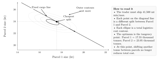
Illustrative form transformation through multi cargo parcel-mix optimisation
Illustrative form transformation through multi cargo parcel-mix optimisation shows form transformation as a practical optimisation problem when considering how to price a voyage. A commodity trader must ship a fixed programme of 41,500 tonnes and decide how much to allocate to Parcel 1 and Parcel 2. Every possible split lies on the diagonal line because the total must always remain 41,500 tonnes. Moving along this line changes the parcel mix while keeping the shipment programme unchanged. The ellipses show total logistics cost for each split. Each contour reflects the combined cost of freight, port handling and operational constraints. The lowest-cost feasible solution is where the fixed cargo line touches the lowest cost contour. In the figure, this occurs at about 17,550 tonnes in Parcel 1 and 23,950 tonnes in Parcel 2.
The trading implication is important. The trader is managing form because the parcel combination must meet the final specification. At the same time, the trader is also managing space and time because different parcels may use different ports, vessel arrangements, loading windows or handling patterns. Illustrative form transformation through multi cargo parcel-mix optimisation therefore shows that a form decision often becomes a combined space-time-form optimisation. The example is theoretical, but it illustrates the tension between the commodity trader's preferred parcel structure and what a shipowner or freight trader can realistically offer. In the spot market, where a suitable vessel is already in position, the available options can be calculated directly. Forward pricing is more difficult because the freight seller will normally require either a premium or flexibility in parcel sizes to accept the freight price risk on behalf of the commodity trader.
Space, Time and Form: The Shipowner's Multi-Leg View
The freight buyer normally prices one cargo movement. The shipowner evaluates a sequence of vessel days. This difference shows space, time and form from the other side of the freight market. For commodity or freight trader, the key question is whether a route price helps the cargo move. For the shipowner, the key question is whether a fixture is the best use of the vessel across its next employment options. The shipowner is therefore not only pricing one voyage, but transforming vessel capacity across space, time and contract form.
A voyage freight rate may be quoted in USD per metric tonne, but the owner does not evaluate the cargo in that unit alone. The owner estimates the gross freight income, deducts voyage costs and converts the remaining income into a time charter equivalent in USD per day. This allows the current voyage to be compared with other employment choices available to the vessel such as a trip time charter, period charter or alternative voyage.
The USD per metric tonne rate still matters because it determines the voyage revenue. However, it is an input into the calculation rather than the final decision measure. The owner's main comparison is the expected daily earnings across the relevant employment horizon.
Every fixture changes three elements of the vessel's position.
It consumes vessel days and determines when the vessel becomes available again.
It moves the vessel to a new region and determines where the next employment begins.
It preserves or removes future cargo choices according to the vessel's physical and contractual form.
This is the shipowner's version of transformation margin. The owner compares the value of fixing now with the value of waiting, ballasting, repositioning or accepting a different contract form. The decision is attractive only if the expected earnings after the fixture exceed the opportunity cost, voyage cost, waiting time and risk allowance.
A voyage paying USD 20,000 per day may therefore be less attractive than a voyage paying USD 10,000 per day. The higher paying voyage may last longer, end in a weak region or cause the vessel to miss a valuable loading window. The lower paying voyage may place the vessel close to a strong next cargo and improve earnings over the full sequence.
This forward looking element has long been recognised in shipping economics. Current employment decisions depend on expectations about future market conditions Z. S. Zannetos (1966). Freight earnings are also stochastic and uncertain rather than known when the fixture is agreed Roar Adland (2003). Regional earnings differences are connected through vessel repositioning, but this takes time because vessels must physically move between markets Roar Adland and Fredrik Bjerknes and Christian Herje (2017).
Owner expectations cannot normally be observed directly. A fixture record shows the agreed rate, route, vessel and contract terms, but it does not reveal the owner's full view of the next market. That view must therefore be inferred from quotations, fixture choices, ballast decisions and later vessel movements.
The following examples isolate the logic across several legs. Each trip is assumed to last 30 days. The FFA reference rises from USD 14,000 per day for Trip 1 to USD 15,000 for Trip 2 and USD 16,000 for Trip 3. This simplified forward curve is illustrative. In practice, the relevant FFA value may vary by month and vessel specification.
Time charter income means each voyage has already been converted into time charter equivalent earnings after voyage costs Martin Stopford (2009). Profit versus FFA means the daily result relative to the FFA reference. It is not the owner's final accounting profit after operating, financing and capital costs.

Table from the book.

Scenario A: Strong first trip earnings, but weak continuation
Scenario A looks attractive on the first trip because the vessel earns above the FFA reference. However, its later trips are weaker, so average earnings over 90 days fall below the benchmark. Scenario B accepts lower earnings on the first trip but positions the vessel for stronger subsequent employment. The lower initial income is therefore a deliberate choice, not necessarily a pricing error. For the shipowner, the example shows that the trade is the complete employment chain rather than one fixture in isolation. The relevant comparison is expected earnings across all vessel days, including ballast, waiting and port time, measured against the corresponding market references. Commodity traders need to understand whether suitable vessels are open in the right region, at the right time and under acceptable contract terms. When this capacity is scarce, freight costs rise and CFR commodity margins tighten.
Why Owners Quote Different Voyage Rates
Building on the scenario from the previous subsection, suppose two owners quote the same voyage cargo at USD 22/mt and USD 26/mt. The USD 4/mt difference does not necessarily mean that the owner quoting USD 26 is unaware of the competing offer. Both owners may know the last fixture, the current broker indications and the approximate level at which competing tonnage is quoting. The difference may instead reflect how each owner values the vessel's space, time and form consequences of the voyage.
The owner quoting USD 26/mt may expect the voyage to create a poor continuation position. In space, the vessel may discharge in a weak region or require a long ballast to the next loading region. In time, the vessel may become open after an attractive cargo window has passed. In form, the cargo or contract terms may restrict the vessel's later employment choices. That owner therefore requires more income on the current voyage to compensate for the expected earnings given up afterwards.
The owner quoting USD 22/mt may hold a different forward view. The voyage may place the vessel close to a strong next cargo, satisfy a redelivery commitment or create access to a region where the owner expects rates to rise. That owner can accept less on the current voyage because the expected continuation earnings make the complete employment chain attractive.
The lowest executable freight offer is therefore not always produced by the owner with the lowest operating cost. It may be produced by the owner who assigns the highest value to the position created after discharge. In practical terms, the cheapest owner may have the cheapest combined valuation of the current voyage and the forward employment chain.
This distinction is important. A low quotation does not necessarily express a weak view of freight. It can express a strong view of where the vessel will be, when it will be open, and what choices remain available after discharge.
Continuation value is not the only reason why owners quote different rates. The difference may also reflect:
Space: the vessel's current position and required ballast cost;
Time: financing needs and willingness to accept near term cash flow;
Form: cargo suitability and port restrictions and existing charter commitments and redelivery obligations;
Cost: bunkers onboard, bunker consumption and technical efficiency;
Execution: contract terms and perceived operational risk; and
Risk: risk appetite and confidence in the forward view;
A freight quotation should therefore be understood as an owner-specific minimum acceptable price under a particular set of costs, constraints and expectations. It is not a statement of one universal value for the voyage.
If one employment chain were expected to produce persistently higher risk adjusted earnings than competing chains, vessels would gradually reposition towards it. The additional vessel supply would reduce the premium in the stronger region. Routes that lost tonnage would need to pay more to attract vessels back. This adjustment tends to equalise expected earnings across several legs, but it does not require every individual trip to pay the same daily rate.
The owner therefore requires more income on the current voyage to compensate for weaker expected earnings over the remaining time horizon. For example, if the voyage occupies the first 30 days of a 90 day planning horizon, the owner may seek a higher spot rate to offset the expected earnings shortfall during the following 60 days. This produces a higher quotation in USD/mt. Owners and charterers may broadly agree on the last concluded spot rate, but that rate does not determine the value of the next fixture to any owner. If the next owner calculates that the voyage would produce lower expected earnings than its competing employment options, it will quote the rate required to bring the complete employment chain closer to parity with those alternatives.
Implication for the Freight Buyer
For the freight buyer, different owner valuations produce a range of quotations, but these quotations are not equally relevant to the immediate purchasing decision. Where vessel quality, contract terms, counterparty risk and execution conditions are comparable, the lowest executable quotation represents the price the buyer can transact at. A higher quotation reveals another owner's minimum acceptable price, but it does not increase the price the buyer needs to pay. If the spread between cheapest and second cheapest is large, this information tells the freight buyer how deep the market is.
It is important that the buyer should understand what the cheapest offer represents. It is the price at which one particular owner is willing to exchange the vessel's present position for the position created after the voyage. A change in expectations about the next regional market can therefore change today's freight quotation even before the physical supply and demand balance on the current route has visibly changed. The freight matrixFreight matrixA table of freight costs by origin, destination, route and shipment month, expressed in a common unit for use in delivered price calculations.Open in terminology records the executable price available to the commodity trader. It does not show the full vessel employment chain behind that price. Understanding this distinction explains why informed owners can quote materially different rates for the same cargo.
This completes the shipowner view of transformation across space, time and form. The next section returns to the freight buyer and shows how executable freight values are combined with FOB prices to construct CFR matrices.
From FOB and freight matrices to CFR matrices
The transformations described above become more useful when they are turned into an operating tool. At the desk level, this tool is often a matrix. A FOB matrix shows the commodity value at each origin and shipment month. A freight matrix shows the cost of moving that commodity from each origin to a destination, also by shipment month. Adding the two matrices in the same unit produces the CFR matrix in FOB and freight matrices combine into a delivered CFR matrix. The space reading is the delivered origin ranking for each month. The time reading is the movement across each row. It is assumed that finance, documents, risk, and margin are roughly the same across origins and destinations..
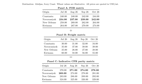
FOB and freight matrices combine into a delivered CFR matrix. The space reading is the delivered origin ranking for each month. The time reading is the movement across each row. It is assumed that finance, documents, risk, and margin are roughly the same across origins and destinations.
The calculation is simple but commercially powerful. A FOB matrix tells the trader the nominal prices at origin and a freight matrix shows the price of freight. The CFR matrix combines the two and shows which origin is the cheapest into that CFR destination. This is where a theoretical supply chain becomes an operational trading decision.
The calculation is not matrix multiplication. It is cell-by-cell addition. Each FOB value must be matched with the correct commodity specification, destination, shipment month and unit. If the FOB value is quoted in USD/mt, then the freight value must also be converted into USD/mt. Only after the units are aligned can the trader compare origins on a delivered basis.
The space signal comes from reading down the matrix within each shipment month. For a given destination and month, the commodity trader can rank all possible origins by CFR. The cheapest FOB origin may not be the cheapest CFR origin. A Black Sea origin may look cheap on FOB, but if freight to the destination is expensive, its delivered value may be worse than a more expensive FOB origin with cheaper freight. Conversely, an origin with a higher FOB price can become the delivered winner if freight is cheap enough.
This is one of the cleanest ways to see how freight shapes global flows. Buyers do not consume FOB wheat. They consume delivered wheat. The destination buyer therefore compares the delivered replacement cost across origins. If one origin becomes cheaper on CFR, demand is pulled towards that origin. If the trade is large enough, that demand can strengthen the FOB prices at the winning origin, tighten vessel supply on the winning route, and force competing origins to lower their FOB basis if they want to compete for demand. Freight therefore does not sit outside the commodity price. It helps decide which surplus region can reach the deficit region competitively.
The time signal comes from reading across each origin row. The trader can compare July, August, September and later shipment months to see which part of the delivered CFR curve is creating or destroying value. If later FOB values are above nearby values, the FOB curve is in contango. If later FOB values are below nearby values, the FOB curve is in backwardation. The same language is often used for freight curves as a trading shorthand, although freight is not storable in the same way as wheat. In freight, the forward curve reflects expected vessel scarcity, route basis, bunker pressure, congestion and the opportunity cost of positioning ships.
The CFR curve combines the time structure of the commodity price and freight. A CFR contango may come from a rising FOB curve, a rising freight curve, or both. A CFR backwardation may come from a falling FOB curve, cheaper forward freight, or a fall in freight that more than offsets a rise in FOB price. This distinction matters because it tells the trader what is actually being traded. If CFR becomes more attractive in a later month because FOB is cheap, the commodity desk owns the view. If it becomes more attractive because freight is cheap, the freight desk owns much of the view. If both move together, the trade is a combined commodity and freight expression.
The CFR matrix is therefore a shared decision map between the commodity desk and the freight desk. The commodity desk uses it to compare origins and shipment months. The freight desk shows how route values, freight basis and the FFA reference affect the delivered price, and which origin is most likely to generate a freight sale.
For the matrix to work inside a commodity company, the freight values must represent the prices that the commodity desk and competing commodity traders would actually pay in the open market. If the internal freight desk skews those values because it prefers to retain a long freight exposure, the CFR matrix becomes distorted. The commodity trader can no longer value the position correctly and may choose the wrong origin or miss a sale. The internal freight trader may nevertheless be right that freight will be several USD/mt higher by the time of execution. In that case, the freight trader and commodity trader must capture the best combined value for the company by buying freight in the open market to facilitate the commodity trader's position.
For the commodity trader, this freight view appears in the CFR matrix as a delivered price. A few dollars per metric tonne in freight can decide whether an origin wins or loses. This is why the freight desk and the commodity desk should work from the same matrix. The commodity trader sees which origin clears the destination. The freight trader sees which route has value relative to paper and relative to competing physical routes. The result is a shared decision map.
The CFR matrix therefore connects the theory of price coordination with the daily work of trading. It answers two operational questions at the same time: where should the cargo move from, and when should the cargo move? The answer is not given by the FOB price alone, and it is not given by the freight price alone. It is given by the delivered price created when both are combined.
A commodity trader should still treat the CFR matrix as a decision aid rather than a contract. Quality, credit, documentary risk, export rules, port performance, vessel suitability and customer preference can all change the executable trade. But the matrix provides the first disciplined view. It converts scattered price signals into one comparable delivered value. That is why freight matrices matter for commodity traders. They show how freight rates and freight basis views become part of commodity allocation, and how prices distribute goods across space and time.
Time and Risk
Transformation margin is calculated before it is realised. The margin is only earned after the cargo, vessel or contract has moved through the execution process. During that period, each stage of the supply chain can change and may have a cascading effect on trade execution. The time lag is the source of execution risk. This is why the formula includes a risk allowance, which is the extra margin required to justify uncertainty.
Delay provides a simple example of how time affects margin in practice. Suppose a trader buys grain inland, charters a vessel and sells the cargo to an overseas buyer for a specific delivery time window. On paper, the transformation margin is positive. However, if the cargo arrives late at the export port, the vessel may wait and incur demurrage which could be for sellers account. The delay may also create extra storage and financing costs. If loading misses the agreed delivery time, the buyer may demand a discount or reject the cargo. The same delay can therefore affect several parts of the formula at once and deteriorate the margin.
Time is therefore a risk multiplier. A space transformation may fail because the freight rises before the vessel is fixed. A time transformation may fail because storage costs increase or quality deteriorates. A form transformation may fail because the adjusted cargo does not meet the specification. The longer the time horizon, the greater the exposure to unforeseen developments.
Property rights and contractual agreements help reduce uncertainty. They define who is entitled to the cargo and payment, who pays for the freight, who carries quality risk and what happens if a party fails to perform. However, contracts do not completely remove execution risk.
Finally, it is useful to distinguish between risk and uncertainty. Risk refers to outcomes that can be estimated with probabilities, such as the likelihood of a shipment delay due to adverse weather. Uncertainty, on the other hand, refers to unpredictable events like sudden policy changes or geopolitical conflicts, which cannot be easily quantified. Both matter for transformation margin, but they are managed differently: risk can often be modelled or hedged; uncertainty cannot be predicted and requires judgement, flexibility and a larger safety buffer.
Identifying Relationships that will Change
The above three levers of transformation explain how value can be created, but they do not by themselves tell the trader which lever to act on. Before cargoes are moved, stored or changed, the trader must first identify a relationship.
Trading strategies and pricing relationships
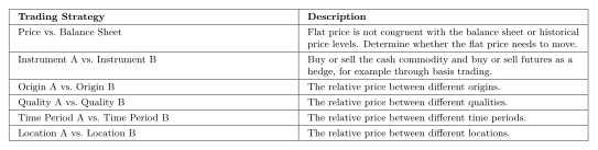
Trading strategies and pricing relationships shows how traders think in terms of price relationships. A flat price may look high or low, but it only becomes meaningful when compared with something else: the balance sheet, another instrument, another origin, another quality, another time period or another location. Trading is therefore not only the activity of buying and selling things. In commodity and freight trading, trading is the identification of relationships that are likely to change, and the allocation of capital to profit from that change.
Each relationship in the first column points to a possible trading question. If flat price looks inconsistent with the balance sheet, the trader may ask whether the flat price is likely to adjust. If Origin A is cheaper relative to Origin B, the trader asks whether cargo can be move between the two markets.
The list is not exhaustive. Rather, it illustrates a method of thinking, i.e. how we can view the world of trading through the lens of relationships that change. Identifying the relationship is the first step. Trading strategies and pricing relationships identifies the relationship. The second step is to test whether it can be executed and converted into margin through space, time and form. This differs from Space, time, and form in physical commodity arbitrage, which shows where value may arise from the three transformation levers.
As seen in Trading strategies and pricing relationships, a margin test applies to all three arbitrage types. The trader buys the commodity in one state, pays the transformation cost, and sells it in a higher-value state. The trade is executed only when the remaining spread is positive after freight, carry, processing, finance and execution risk. Below are some test examples for each lever.
Spatial arbitrage. A trader buys wheat FOB Origin A at USD 242/mt and sells it CFR Destination B at USD 264/mt. Ocean freight and finance total USD 20.7/mt. Net margin is:
The USD 1.3/mt is the trader's remaining margin before the risk allowance. The trade is attractive only if the trader can secure all costs at levels that leave an adequate expected margin after accounting for the full position. Any additional cost above USD 1.3/mt eliminates the margin on this trade unless it is offset by gains elsewhere. In practice, a trader may still accept a low-margin or loss-making trade if it creates valuable optionality, builds volume or provides access to subsequent arbitrage opportunities.
Temporal arbitrage. A trader buys barley after harvest at USD 218/mt and sells three months forward at USD 227.4/mt. Storage, finance, insurance and shrinkage total USD 8.0/mt. Net margin is:
The trade is viable only if silo capacity, credit and quality preservation are available. Sometimes the scarce asset is not the barley itself, but storage and port capacity. In that case, booking capacity can become part of the trade.
Form arbitrage. A trader buys one high-quality wheat parcel at USD 300/mt and one low-quality wheat parcel at USD 200/mt. A 50:50 blend gives an input cost of USD 250/mt and can be sold as a medium-quality cargo at USD 255/mt. Blending, testing, handling and shrinkage cost USD 3.5/mt. Net margin is:
The USD 1.5/mt is the value created by converting two separate qualities into a cargo that better fits market demand. The trade only works if the blended cargo meets the contractual specification. In practice, form arbitrage often overlaps with space and time because cargoes may be bought from different origins, stored across different periods and blended at destination.
The examples show why physical arbitrage is usually a narrow margin business. A positive spread is only an initial indication of value. The trade remains attractive only if the margin is sufficient to absorb operational constraints, capacity bottlenecks, contractual obligations and execution risk. The trader must therefore test not only whether a price relationship appears favourable, but whether it can be converted into a reliable and executable profit.
The Power of Optionality
Optionality is a pivotal concept in trading. An option gives the holder the right, but not the obligation, to buy or sell an underlying asset, or to receive a cash settlement, under specified conditions. The buyer pays a premium for this flexibility and exercises the option only when doing so is beneficial. This flexibility may be undervalued in traditional discounted cash flow analysis.
Optionality changes the commercial result while leaving spread uncertainty unchanged. Note that the action and result depend on whether the trader is long or short a call or put option. shows how optionality changes the payoff while leaving spread uncertainty unchanged. A rigid contract forces the trader to execute in both states: if the spread widens, the trader captures the upside; if the spread collapses, the trader must absorb the loss. In contrast, an optional contract gives the trader the right, but not the obligation, to execute. The trader exercises when the spread widens and walks away when the spread collapses. The cost of this flexibility is the premium. Optionality therefore keeps the upside open while limiting the downside to the premium paid. When spreads become more volatile, this flexibility becomes more valuable because adverse moves are capped, while favourable moves can still be captured. In physical commodity trading, optionality manifests through various routes.
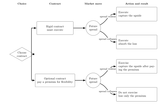
Optionality changes the commercial result while leaving spread uncertainty unchanged. Note that the action and result depend on whether the trader is long or short a call or put option.
Cash-and-Carry Trades: When futures markets are in contango, where future prices exceed spot prices, traders can buy the commodity at the lower spot price, store it and sell it at the higher future price, locking in a spread. Profitability depends on whether the spread exceeds storage and financing costs. The optionality comes from control over storage.
Pricing Period Optionality: Traders might negotiate contracts allowing them to choose the pricing month for shipments within a specified range (e.g., Month M or Month M+1). This flexibility lets them exploit calendar spread movements without immediate commitment. If the market shifts from contango to backwardation, where future prices are lower than spot prices, the trader can adjust their pricing periods to maximise gains. The value lies in the right to choose timing.
Exchange Arbitrage: Similar commodities traded on different exchanges may show temporary price discrepancies. A trader can buy the cheaper contract and sell the more expensive contract, but the apparent spread is executable arbitrage only if it exceeds all delivery, quality conversion, currency, financing and transaction costs. Otherwise, the position is a relative value trade with basis and convergence risk, not a locked arbitrage.
Physical Assets as Options: Owning assets like storage facilities or processing plants imbues traders with inherent optionality. For instance, owning storage allows traders to capitalise on high storage fees during oversupply periods. They can choose to use the storage themselves or rent it out at elevated prices. This strategy aligns with the real options theory in economics, where investing in physical assets provides flexibility to respond advantageously to market changes.
These examples show that optionality is not separate from transformation. It gives traders more choices over how to use space, time and form. The more flexible the trader is, the more routes are available for capturing transformation margin when market conditions change.
Trading Events and Margin Shocks
Most trading portfolios contain several sources of risk. Some of these risks can be reduced inside the book because exposures offset one another. However, not all risks can be diversified and internally neutralised. Some risks come from outside the portfolio and change the market itself. These discrete external shocks are called trading events and the exposure they create is event risk.
This often stems from geopolitical factors. Events such as trade embargoes, canal closures, war, political unrest, or changes in export policies can significantly impact supply and demand dynamics. Event risk matters for transformation margin, as it can change the formula suddenly. When new information emerges, the market rapidly seeks a new equilibrium. Prices adjust swiftly as traders reassess expectations, reallocating capital in response to updated information. This dynamic highlights the importance of being well-informed and prepared to interpret how events will affect prices.
Relative prices move faster than capacity shows the trading window created when relative prices move faster than physical capacity can respond. From left to right, beliefs are priced in, new information moves relative prices, physical reallocation lags, and spreads narrow as capacity catches up. The gap between the price move and the slower physical adjustment creates the trading window.
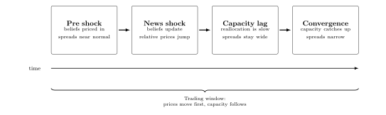
Relative prices move faster than capacity
A critical concept in trading event risk is understanding what is "priced in": the market's current expectations based on all available information. Prices reflect not just known facts but also collective anticipations of future events. For instance, if a drought in a major wheat-producing region is widely anticipated, its potential impact on supply may already be factored into current prices. By contrast, an increase in piracy in the Gulf of Aden, a War in Ukraine or Houthi's shooting rockets at commercial ships are not. There are theoretically three strategies for trading event risk Brent Donnelly (2021):
Before it happens: Taking a view into the event: Traders may form a strategic position ahead of a known event, such as a government report on crop yields. By analysing economic indicators and employing mathematical models they estimate potential outcomes and position themselves accordingly. Risk monitoring is essential here as unforeseen results can lead to significant losses.
While it happens: Positioning your book for different outcomes: Traders might deem some of the risk of the event priced in. An example could be if there is a semi-hot war in Gaza, but traders might think that the price of buying, e.g. call options on oil, looks attractive as a small escalation of the war could involve Iran and Saudi Arabia putting a large part of the world's oil supply at risk.
After it happens: Re-evaluation of Prices: Sometimes the market may overreact to news, leading to price movements that are unsustainable in the short term. Traders can see this overreaction and take positions against the prevailing trend when it happens, expecting prices to revert as the market corrects itself.
In all strategies, risk management is central. Traders must consider factors like market liquidity, potential price gaps and the limitations of their predictive models. They often use hedging instruments and diversify their portfolios to mitigate adverse effects.
Trading or Merchandising?
Not all traders are alike; the swashbuckling days of Marc Rich traversing the globe for quick profits are over. Today's traders tend to specialise, investing heavily in knowledge, relationships and infrastructure within specific niches of commodity markets. This specialisation has led to siloed roles. In some large trading houses, while teams are called "traders," strategic decisions rest with the desk head; the rest execute strategies with limited autonomy Luc Nijs (2014). Merchandising creates value through reliable execution of committed flows. Trading creates value through preserving and exercising flexible rights under hard constraints. distinguishes merchandising from trading: merchandising executes committed flows, while trading preserves and exercises flexible rights under constraints.
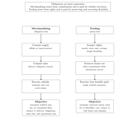
Merchandising creates value through reliable execution of committed flows. Trading creates value through preserving and exercising flexible rights under hard constraints.
Merchandising has become central not only to commodity flows, but increasingly to freight as well. Many trading firms secure long-term offtake agreements that guarantee a steady stream of product, offered at discounted prices because the trader provides prepayment or financing deals. This creates recurring physical purchase commitments for trading houses, although their net price exposure depends on their sales and hedges. The effect is reinforced when agricultural commodity trading companies own production assets. While this can be beneficial in rising markets, it poses challenges when markets soften.
In this setting, merchandisers must logically sell at the best possible price while minimising logistics costs and operational disruptions. Success hinges on reliability and strong consumer relationships, not just market intuition. Despite commodities being standardised, relationships matter. Many consumers run minimal inventories to reduce costs, so timely delivery and exact specifications are critical. Delays or off-spec materials can cause significant disruptions due to tight production tolerances and costly disposal of harmful by-products.
Thus, a merchandiser's core task is to ensure supply chain reliability which is typically achieved through the close coordination with the head trader. By consistently fulfilling customer needs without problems, a merchandiser can build a successful career in the commodity industry without having to be a speculative genius. A notion that might just lighten the mood for those interested in the commodity business but valuing stability over thrill.
Trading is fundamentally a team sport, where success depends on coordinated execution and effective communication. Regardless of individual roles, each team member's contribution is essential. Shared insights, joint risk management and collective decision-making ultimately determine trading outcomes, emphasising the importance of teamwork in navigating complex and dynamic market environments.
Carry the model forward.
Key Takeaways
Freight and commodity trading share much of the same underlying economic logic, even if their instruments differ.
Traders create value by moving, timing and reshaping flows better than competitors.
Optionality is valuable because it preserves future choices under uncertainty, but often comes at a price.
The best trades often arise from recognising which relationships are about to change before they do - and before competitors realise they will change.
Connection to the Next Chapter
This chapter shows where trading edge can come from. The next chapter shows how such market views can be monetised through basis trading.
Continue to Basis Trading