Balance Sheets
Jump to a section2 sections in this chapter
Balance Sheets
Traders form a view on whether to buy or sell in the market by analysing the supply vs. demand balance. In trading jargon, this is a balance sheetBalance SheetIn trading, a market accounting framework that organises available supply, expected demand and the resulting surplus or deficit over a defined period.Open in terminology. It is not an accounting balance sheet that records the assets, liabilities and shareholders’ equity of a company at a specific point in time. A trading balance sheet is a market accounting framework. It tracks available supply, expected demand, and whether conditions are tightening or loosening.
In commodity markets, traders track a small set of core variables: production, imports, exports, consumption, stocks and trade flows. Putting these pieces together gives a directional view of the market surplus or deficit. Because markets tend to clear locally before they clear globally, balance sheets are best treated as dynamic and regional. Weather conditions, government policies, and substitution can quickly shift the balance.
The same logic applies in freight markets, but "stocks" and "flows" are different. Freight traders do not track inventory directly. Instead, they track transport capacity through vessel positioning, congestion, fleet supply and tonne-miles demand for freight services. From commodity fundamentals to freight clearing. Commodity fundamentals determine net trade requirements, which are translated into seaborne allocation and routing, trade stems, and demand for shipping services measured in tonne miles. Freight rates then clear transport demand against open tonnage and the marginal ship's reservation level. shows how commodity imbalances translate into the freight balance sheet. Commodity fundamentals determine a net trade requirement; that requirement becomes tonne-mile demand for shipping services. Freight rates then clear transport demand against open tonnage and the marginal ship's reservation level.
Tonne miles equal cargo metric tonnes multiplied by sailing distance. The math is simple: cargo mt multiplied with sailing miles equals tonne-miles Martin Stopford (2009). For a 60,000 mt Panamax soybean cargo to Shanghai, a Santos voyage of roughly 12,500 miles generates about 750 million tonne-miles, while a Pacific Northwest voyage of roughly 5,700 miles generates about 342 million. The Brazilian cargo therefore creates more than twice the transport demand despite moving the same volume. The longer haul occupies the vessel for more days, delays its next open position and absorbs fleet capacity. Freight balance sheets should therefore track changes in sourcing patterns, not merely aggregate soybean exports, because origin determines effective demand for ships.
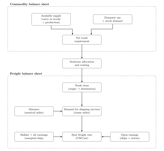
From commodity fundamentals to freight clearing. Commodity fundamentals determine net trade requirements, which are translated into seaborne allocation and routing, trade stems, and demand for shipping services measured in tonne miles. Freight rates then clear transport demand against open tonnage and the marginal ship's reservation level.
The purpose of this chapter is to make the balance sheet logic transferable. The goal is not perfect forecasting, but disciplined forecasting based on market intelligence: to be consistently less wrong than the market and to understand which variables drive outcomes under different regimes. Once we foresee a tightening or loosening market, the next step is translating that view into price expectations and managing the associated risks.
Balance Sheets in Commodity Trading
In commodity trading, a balance sheet is a structured accounting of physical availability over a defined period, typically a marketing year. Traders track inflows (beginning stocks, production and imports) against outflows (domestic consumption and exports), with ending stocks as the residual.
The inflow side and the outflow side are driven by different forces. Commodity demand also changes over different time horizons. Cyclical demand reflects short-term movements caused by price changes, income conditions or inventory behaviour. Structural demand reflects medium-term shifts in consumption patterns, processing capacity, trade policy or substitution. Secular demand reflects long-term forces such as population growth, economic development and dietary change Daniel Ahn (2019). For balance sheet work, the practical question is how these demand shifts affect domestic use, imports, exports and ending stocks.
Agricultural products have features that make their balance sheets different, adding a further complication to the balance sheet. Agricultural supply is biological and seasonal. Before planting, farmers decide how many acres to dedicate to each crop based on competing crop prices and pre-plant weather conditions. These decisions set the baseline production potential. After planting, supply becomes difficult to adjust in the short run and outcomes depend largely on yields, with post-plant weather often the dominant driver. Government policies matter too: price guarantees, subsidies and crop insurance programmes can affect incentives and shift planting decisions across crops.
Many agricultural commodities are both seasonal and storable, with inventories acting as a buffer that absorbs shocks and determines how tight the market becomes. Balance sheets are therefore organised around the marketing year, starting with the first month of harvest and ending with the following year's harvest and typically segmented by commodity type, country and region Luc Nijs (2014). Forecasting begins nearly a year in advance, incorporating both northern and southern hemisphere production to account for global supply variations. It is worth noting that even with careful accounting, uncertainties remain: demand can shift, trade policies can alter and stock information is often reported with a lag, leading to ongoing market speculation and potential price volatility.
The structure described above is easiest to see in grains such as wheat, corn or soybeans. However, commodity markets are not uniform. Differences in production cycles, quality specifications and seasonality can require a different accounting structure even when the underlying logic is the same. To highlight this, the next subsection introduces sugar, an important bulk commodity with a very different market structure.
Sugar vs. Grain Balance Sheets
Unlike most grains, sugar production is spread more evenly throughout the year and is heavily influenced by the southern hemisphere, which accounts for about 60% of the world's raw sugar exports Jonathan Kingsman (2000). As a result, sugar balance sheets are often built as a 12-month flow analysis rather than through a single crop-year snapshot. Practitioners often break the year into quarters or months to maintain a more nuanced understanding of supply and demand dynamics.
Sugar also requires analysts to be explicit about quality. The market differentiates between raw sugar and white sugar, requiring quality conversions and adjustments based on factors such as polarisation and local definitions. For example, raw sugar often needs to be converted to a standard polarisation level, adding another dimension to the data analysis.
On the supply side, sugar production has a process called ratooning, in which sugar cane regrows after harvest, allowing multiple harvests before replanting. This ratooning therefore introduces longer-term supply cycles (six to eight years); consequently, the supply response to price signals can play out over multiple seasons rather than within a single year.
The practical takeaways are not that sugar is "harder" than grains but that the same balance sheet logic must be implemented differently. Compared with grains, sugar balance sheets tend to be more sensitive to timing and to quality and they often require more conversion work to harmonise data across sources. In addition, analysts must integrate data from multiple countries with differing reporting standards and account for seasonal and cyclical production factors unique to sugar.
Balance Sheets in Freight Trading
In freight markets, traders often estimate effective supply from open tonnage adjusted for speed, congestion, port turnaround time and idle days. Transport demand is measured by cargo volumes and the tonne-miles required to move them. However, the freight balance sheet is rarely “global supply vs. global demand.” It is a matching problem: corridor-specific transport demand must be met by the right pool of ships in the right place at the right time.
A practical way to structure this matching problem is by vessel segment because each segment competes in a different arena and clears on different information sets. For example, Capesize vessels operate in a largely global market, dominated by long-haul iron ore and coal flows that link major exporters such as Brazil and Australia with demand hubs in Asia. Panamax vessels, sized to pass through the Panama Canal, typically clear more at the basin level, moving commodities such as grains and minerals within the Atlantic and Pacific basins, often servicing routes between continents but within specific oceanic regions.
Smaller vessel classes provide greater regional and port flexibility. Supramax vessels trade globally but are particularly useful on regional and interregional routes, carrying cargoes such as fertilisers, cement and grains. Their size allows them to call at a wider range of ports than larger bulk carriers. Handysize vessels offer even greater flexibility, serving smaller ports, niche routes and fragmented cargo programmes that larger vessels cannot access efficiently. Each vessel segment therefore has its own balance sheet although there are overlaps: demand is shaped by relative prices between vessel sizes, cargo volumes, parcel sizes and timing requirements, while supply depends on the number of suitable vessels that are commercially open and correctly positioned. Consequently, one vessel segment or region can tighten while another remains well supplied. Where operationally feasible, freight buyers may respond to relative freight costs by dividing cargoes into smaller parcels or switching between vessel classes.
Forecasting with Balance Sheets
For traders, forecasting freight rates and market conditions is a necessity to compete. Every decision; whether to charter a ship, order a new vessel, or divest an existing asset, relies on the view of future conditions Martin Stopford (2009). The purpose of the balance sheet, however, is not to predict the rate. It is to translate scattered signals and indicators into a disciplined view of tightening or loosening and to update that view quickly when market changes.
Balance sheets do this by imposing a clear structure at the level where freight markets actually clear. They break demand down into corridor and segment-specific cargo types and translate volumes into tonne-mile requirements. For instance, these balance sheets model individual countries' seasonal demand for specific cargo types, account for regional crop cycles and track the precise location and status of ships to match demand with shipping capacity in near real-time. This approach is valuable because shipping forecasts have a poor record when they are treated as precise point predictions. In freight trading, the edge comes from sharper real-time monitoring, which makes balance sheets more suitable for operational decisions in commodity supply chain logistics. A good balance sheet is therefore a living model, simple enough to update daily, but structured enough to capture the market dynamics.
Traditional cycle indicators still matter as context. Fleet growth, scrapping, speeds, and global trade growth help define the background regime and the plausible range of outcomes over time Martin Stopford (2009). But the balance sheet lens is what turns that backdrop into an actionable trading map by identifying where the market clears in practice: specific corridors, specific segments, and specific timing constraints.
Foreign Exchange
Foreign exchange (FOREX) dynamics are central to commodity trading and therefore freight trading. From a balance sheet perspective, FOREX is one of the variables that can move the trade flows from one origin or destination to another. FOREX rarely alters production or the harvest itself, but it changes the local currency economics of selling into a market priced in USD and thus the competitiveness of an exporter's offer. That shift affects who becomes the marginal exporter, how quickly an origin sells and where cargoes are routed. In other words, FOREX moves the balance sheet by changing the pace at which a surplus clears and the direction in which trade flows move.
Consider a European commodity trader exporting grain to Asia under contracts priced in USD. If the EUR strengthens against the USD, the EUR value of the trader's USD receipts falls. In this case, margins tighten, the trader's incentive to sell weakens and flows may shift to alternative origins with more favourable currency economics. These FOREX-driven changes appear directly in the balance sheet through exports and feed into the freight balance sheet by changing volumes, corridors and tonne-mile demand.
FOREX becomes most operationally binding when trades are executed on CFR terms because the trader is managing a combined position across commodity, freight and currency. Under CFR, the delivered price is committed, while the FOB goods and freight must be secured and the derivative positions executed before the combined position can be considered hedged.
Working capital and liquidity in a CFR trade under a sight letter of credit. Solid arrows show the sequence within each band. Dashed links show dependencies across the commercial cash cycle, bank finance and hedge liquidity. Payment timing differs under CAD, usance LC and open-account terms. shows the working-capital and liquidityLiquidityThe ease with which an agricultural commodity such as wheat can be bought or sold in the market.Open in terminology cycle in a CFR trade. The first band shows the commercial cash sequence, the second the bank-finance sequence, and the third the hedge-liquidity sequence. Under a letter of credit, cash is committed when the seller purchases the FOB cargo and fixes or pays freight, but payment for the cargo is normally released once the bank has received and checked a complying presentation of clean documents evidencing shipment on board. The cash cycle is therefore much shorter than the physical voyage. Under CAD, documentary collection, LC or open-account terms, however, the seller’s credit exposure may continue until buyer payment or maturity. The balance sheet issue is therefore not only the physical cargo value, but the timing mismatch between purchase finance, freight payments, LC proceeds and hedge liquidity. Futures, FFAs and FOREX hedges may require initial margin, variation margin or collateral before trade cash is received. A profitable trade can therefore still become liquidity-constrained if bank lines, margin calls or collateral requirements exceed available headroom.
Traders manage FOREX risk with standard instruments such as forwards, options and swaps. For example, a European trader selling in USD can use a forward to lock a EUR/USD rate and stabilise the EUR value of expected sales proceeds. FOREX hedging therefore not only secures margin; it also helps keep the export programme executable and the cash cycle stable. FOREX interacts with the other two pillars of a CFR offer: FOB and freight. FOB is influenced by local cost structures and the local currency; freight is driven by corridor-specific vessel supply and tonne-mile demand. When currencies, FOB, and freight move in the same direction, pricing pressure compounds. A strong EUR alongside rising freight, for example, can compress delivered margins quickly and force the trader to re-price, re-route, or delay execution. For balance sheet work, the key is that these pressures do not remain “financial.”
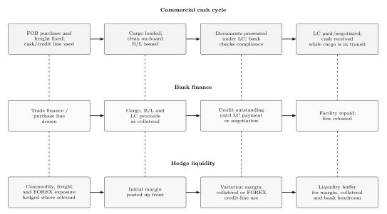
Working capital and liquidity in a CFR trade under a sight letter of credit. Solid arrows show the sequence within each band. Dashed links show dependencies across the commercial cash cycle, bank finance and hedge liquidity. Payment timing differs under CAD, usance LC and open-account terms.
Research shows Theodora Bermpei and Leonardo Ferrara and Andriana Karadimitropoulou and Andreas Triantafyllou (2024) that exchange rates of commodity-exporting countries, often termed "commodity currencies," are influenced not only by individual commodity prices but also by uncertainty across a basket of commodities. An increase in global commodity price uncertainty triggers short-term depreciation in the effective exchange rates of commodity currencies, followed by a medium-term recovery. This pattern is specific to commodity currencies and is not observed in benchmark currencies such as the EUR and USD. The cited study finds that the EUR tends to be neutral to such shocks, while the USD acts as a typical safe-haven currency during periods of market volatility. This phenomenon, termed the "commodity uncertainty currency" property, highlights how commodity price volatility impacts exchange rate dynamics in exporting countries. The findings underscore the sensitivity of commodity currencies to global commodity price shifts, especially during periods of heightened uncertainty.
How Balance Sheets Shape Prices
The previous section introduced the balance sheet as a way to form a view of the market. This section decomposes the balance sheet and shows how those factors work in freight trading. Freight formation as a comparison between two outputs. summarises the structure in two layers. The macro horizon provides the reference level, while the regional horizon determines the spot route rate. The gap between them is the route basis. In practice, the freight trader’s task is to identify whether the regional balance sheet differs from the broader market reference and whether that difference is already reflected in price.
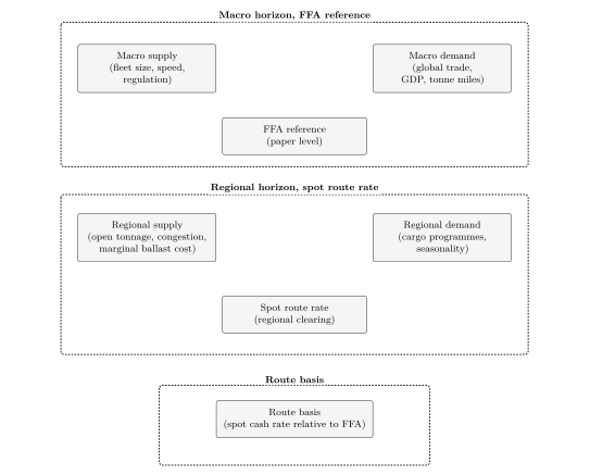
Freight formation as a comparison between two outputs.
Macro Horizon Inputs
Macro inputs provide the reference layer of the freight balance sheet. They do not usually determine which ship fixes the next cargo, but they help explain the broader level reflected in FFA pricing. In this sense, the macro layer is not the final trading answer; it is the benchmark against which the regional balance is compared.
On the supply side, the relevant macro inputs include fleet size, newbuilding orders, scrapping, vessel age, average speed, regulation and technical efficiency. These variables shape the potential transport capacity available to the market. Shipping supply changes slowly because vessels take years to build, so macro supply is more stable than agricultural production. However, small differences in fleet growth can still matter over a cycle, especially for shipowners and investors making long-term asset decisions. Macro supply is not only a question of how many vessels exist, but also how efficiently that fleet can operate. Average speed, technological efficiency and regulation all affect the effective transport capacity available to the market. Global shocks such as geopolitical tensions, pandemics and environmental rules can further alter the macro balance by changing fleet deployment, operating costs or the retirement profile of older ships.
On the demand side, the main macro inputs are global trade, GDP growth and industrial production, which together shape commodity demand. The seaborne share of that demand generates cargo volumes, which become tonne-mile demand once distance is included. Traders may take positions based on expected freight demand through buying and selling of FFAs, COAs or period tonnage. Tonne-mile demand is an especially important metric because it combines volume and distance. A rise in commodity volume does not affect freight equally across all routes. One tonne shipped across oceans creates more vessel demand than one tonne moved within a nearby region. Policy and structural shifts also enter the macro demand layer. Tariffs, trade agreements, environmental regulations and sustainable preferences can change the volume, direction and distance of trade flows. For example, a shift in soybean sourcing due to tariffs can change panamax tonne-mile demand even if total demand is unchanged.
The macro inputs define whether the broader freight market is priced for stronger or weaker utilisation, but the trader must still test that reference against the regional balance: which cargoes are appearing, where they are going, and which ships they require.
Regional Horizon Inputs
While the macro layer provides the reference level, the regional layer tests whether that reference holds for a specific corridor, vessel segment and shipment window.
On the supply side, the main regional input is effective open tonnage. It is the number of commercially available ships that can meet a cargo's shipment window within specific geographic areas. In addition to availability and position, operational factors such as vessel draft, emissions compliance, speed and status (laden, in ballast or idle) also affect effective capacity. A ship may exist in the global fleet but still be irrelevant to a specific cargo if it is too far away, already committed, or unsuitable for the port.
This is why spatial distribution matters more than the macro metrics such as order books and fleet size. A global fleet may look balanced while one basin is tight and another is oversupplied. For instance, a concentration of ships in the Pacific with a scarcity in the Atlantic can lead to favourable rates for owners in the Atlantic, while owners in the Pacific may face diminished rates. Automatic Identification System (AIS) can help traders monitor vessel locations and movements Roar Adland (2021). A theoretical comparison of current AIS ship counts with historical averages could, for example, show the following:
Handysize vessels are evenly distributed across regions, with a lower than seasonal average for ECSA.
The ratio of Supramax ships in the Pacific versus the Atlantic remain relatively stable, although there is a noticeable incrase in ships on the West Coast AMericas.
Panamax vessels in the Atlantic are significantly below the historical average, with 18% fewer ships than usual.
These patterns help traders to make informed decisions to optimise vessel positioning and capitalise on regional rate differentials. Nevertheless, AIS data must be interpreted carefully because of data noise and the difficulty of distinguishing between laden ships, ballast voyages and transient movements. Data providers sell clean data, but this comes at a premium price.
On the demand side, regional inputs are cargo programmes, which are shaped by local production, industrial activity, trade relationship and seasonality. For instance, China's steel sector drives substantial demand for geared ships, while resource-rich areas like South America require bulk carriers for transporting minerals and agricultural products to China. Agricultural exports often peak around harvest windows, while industrial flows depend on local output, processing margins and import demand. Regional policies, infrastructure constraints and port capacity can also affect whether cargoes move smoothly or are delayed.
For balance sheet work, the key is to translate these regional drivers into measurable indicators covering monthly or weekly volumes. A South American balance sheet might track exports of iron ore, steel products, corn, soybeans and sugar using historical data and forecasts, while also assessing which Handysize, Supramax or Panamax vessels are suitable and commercially open. The trader's task is to identify an imbalance between cargo demand and effective open tonnage before it is fully reflected in price.
Route Basis
Route basis is the difference between the regional spot route rate and the broader macro reference. It appears when the local supply-demand balance diverges from the broader market. If a regional balance tightens faster than the macro market recognises, the spot route may strengthen relative to the reference level. If local tonnage is abundant while broader market remains firm, the route may trade at a discount.
The balance sheet question is therefore not simply whether the basis is high or low, but what local supply or demand condition is causing the regional route to trade away from the macro reference. Basis also matters because it can trigger adjustment. Higher regional rates may attract ballast tonnage from other basins, while also testing cargo demand through delayed shipments, origin shifts, parcel-size changes, or vessel-class substitution. These responses can narrow or widen the gap over time, which is why the balance sheet must be updated continuously.
When freight rates in Region A increase significantly, it becomes economically attractive for shipowners in Region B to send their vessels to Region A, even after considering the additional ballast costs. This price-driven movement ensures that ships are allocated to regions with higher demand, optimising fleet utilisation and maintaining market equilibriumMarket equilibriumA price and quantity, or set of prices and quantities, at which planned supply and planned demand are mutually consistent under the relevant market rules and constraints. Equilibrium does not imply that prices are constant or that the market is free from shocks.Open in terminology. By incorporating ballast costs, freight rates effectively incentivise shipowners to respond to regional disparities, allowing the global fleet to adjust dynamically to shifting economic conditions.
Freight demand can adjust through reallocation, substitution and, in some cases, genuine demand destruction. If a commodity becomes cheaper to source from Region B than from Region A, buyers may change origin. This reduces freight demand on routes from Region A but increases it elsewhere; depending on voyage distance, it may also increase or decrease total tonne-mile demand. Buyers can also alter parcel sizes or switch vessel classes when relative freight rates, port restrictions and cargo availability make another option more economical. For example, a buyer may replace one Panamax shipment with several Supramax shipments, shifting demand between vessel segments without necessarily reducing aggregate cargo volume. Genuine demand destruction occurs when freight costs make the underlying commodity trade uneconomic, causing shipments to be delayed, reduced or cancelled. This lowers the quantity of freight demanded at prevailing rates and may reduce freight rates and fleet utilisation, but it does not necessarily represent a permanent shift in the demand curve.
The interplay between supply creation and demand destruction ensures that freight markets remain responsive to both global and regional economic conditions and also makes modelling a repeat task. Shipowners must continuously monitor supply, demand and price signals to adjust their fleet deployment strategies to align with market demands, while freight buyers navigate cost pressures and sourcing decisions that influence their freight needs. Short run fleet supply is relatively flat at low utilisation and steep near capacity. As demand rises from \(D_1\) to \(D_2\), equilibrium moves from \(E_1\) to \(E_2\). Quantity increases modestly, from \(Q_1\) to \(Q_2\), but freight rates rise sharply, from \(P_1\) to \(P_2\), because spare capacity is limited. shows why freight rates can rise sharply near capacity: quantity adjusts only modestly once spare fleet capacity is exhausted.
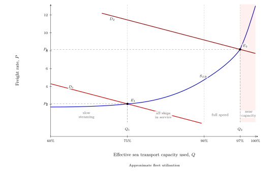
Short run fleet supply is relatively flat at low utilisation and steep near capacity. As demand rises from \(D_1\) to \(D_2\), equilibrium moves from \(E_1\) to \(E_2\). Quantity increases modestly, from \(Q_1\) to \(Q_2\), but freight rates rise sharply, from \(P_1\) to \(P_2\), because spare capacity is limited.
The Trading Opportunity Framework (TOF)
An analyst's job is not only to understand markets but also to formulate trading ideas that a trader can price, hedge and execute. There exist no formal education nor model to do this right. It is about communicating the essentials so that the trader can easily grasp what the opportunity for a trade is, and how the mechanics of it works. The Trading Opportunity Framework (TOF) below is a novel five-step framework for turning an opportunity into a trading plan, but given the flexibile nature of the written word, it can easily be amended to include extra steps if deemed necessary:
Opportunity
The first step in capitalising on any trading opportunity is to clearly define what the opportunity entails, i.e. which relationships are "off". This involves a thorough analysis of the market conditions, identifying anomalies that present a trading opportunity. For instance, in the freight market, an opportunity might arise from an unexpected surge in demand for shipping routes between specific ports due to geopolitical events, a bumper harvest or economic shifts. By precisely outlining the nature of the opportunity traders can focus their efforts on strategies that leverage these unique market conditions, ensuring that their actions are targeted and effective.
Hedging
Once the opportunity is identified, it is crucial to isolate it from unrelated exposure to ensure that potential gains are not offset by unforeseen adverse movements. An example would be a basis trade (in freight markets, this would involve selling a physical voyage and buying FFAs) in which the analyst expects the basis to narrow. Hedging out extra risks such as emissions, currency and fuel price risks reduces the overall risk of the venture. By mitigating these ancillary risks, traders can maintain a clear focus on the primary opportunity, enhancing the likelihood of realising the expected returns.
Risks
Every trading position carries inherent risks and it is essential to anticipate events that could render the opportunity unfavourable. Traders must develop robust exit strategies to protect their investments in case the market dynamics shift unexpectedly. This involves identifying specific triggers that would prompt an exit, such as significant changes in demand, geopolitical instability or adverse weather conditions affecting shipping routes. As soon as the trade is in the book, the risk management process starts.
Profit and Exit
Traders must evaluate how far a trade can go, whether in their favour or against them. If, by day three, the market has moved significantly beyond expectations, it may be time to take profit. However, trading is inherently dynamic, requiring traders to regularly reassess their strategies. A prudent trader outlines plausible scenarios and continuously revisits them, adapting to changing market conditions.
Exit strategies are equally vital. Traders must consider the anticipated costs of exiting a position, including transaction fees or potential losses. Being aware of these factors allows traders to make informed, prompt decisions, thus minimising the negative impact on their portfolio. Exit strategies should not be static; they must evolve alongside market conditions to safeguard profits and manage risks efficiently.
Execution
The final component of capitalising on a trading opportunity is the execution strategy, which outlines how the trades will be implemented to achieve the desired outcomes. This involves determining the timing, scale and methods of entering and exiting positions to optimise performance. For instance, in the freight market, an execution strategy might include a go-to-market strategy of using shipbrokers, utilising real-time data to adjust positions based on market feedback and employing automated indicators to be able to respond swiftly to changes. A well-crafted execution strategy ensures that the theoretical opportunities are translated into practical actions, allowing traders to efficiently manage their portfolios and achieve sustained profitability.
Carry the model forward.
Key Takeaways
A balance sheet is a disciplined way of organising market evidence, which will help increase the odds of making the right predictions, but it is not a prediction machine on its own.
Freight balances differ from commodity balances because freight is a transport service rather than a storable physical good. This distinction changes the economic fundamentals of trading freight markets.
Regional tightness, global demand and global fleet conditions must be analysed together as everything is connected by price.
Good analysis requires both numerical structure, clear written judgement and communication skills.
Connection to the Next Chapter
Balance sheets identify where the market may be tight or loose. The next chapter explains where that value comes from in the first place: transformations in space, time and form.
Continue to Space, Time and Form